NG-mVPN is a next-generation multicast distribution technology that is predominantly used in service provider networks and addresses scalability and manageability issues associated with the previous generation of SP Multicast VPN (Draft Rosen).
In this article, we will go through configuration steps you’d need to undertake to configure NG-mVPN in a Juniper environment. We will also discuss BGP advertisements that are associated with multicast sources and receivers connected to the network. Continue reading “Next Generation Multicast VPN (NG-MVPN) configuration example”
Hot Potato and Cold Potato are two practices of exchanging traffic between BGP Peers. The difference in these two methods is in the approaches to how to carry traffic across the network.
Hot Potato vs Cold Potato discussions are only relevant in the scenarios where multiple traffic exchange (peering) points exist between two networks.
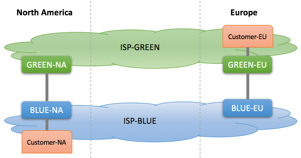
In our example, we will use the following diagrams depicting two networks spanning across North America and Europe.
We are interested in the traffic flow that is originated by Customer-NA connected to ISP-BLUE and is destined to Customer-EU connected to ISP-GREEN.
As the name suggests, BGP-Free Core is a network deployment approach where Service Providers’ Core routers do not run BGP. This is done by employing a tunneling mechanism of some sort, most commonly MPLS.
What are the advantages of a BGP-Free Core?
There are many, to list just a few:
Core devices do not need to be capable of supporting a large number of IPv4/IPv6 routes, allowing you to deploy devices with limited RIB and FIB Capacity
As there is no BGP, Core devices will not be impacted by BGP-related issues, such as high CPU utilization during massive BGP re-convergence
By not running BGP, you eliminate one of the attack vectors – if a new BGP security vulnerability were to be discovered, Core devices would not be impacted
Operators’ mistakes associated with BGP configuration can be eradicated
New services such as MPLS VPN, IPv6, EVPN can be introduced without modifying the Core routers
If deployed properly, BGP-Free becomes unreachable from the Internet, making DDoS and hacking attacks against ISPs’ Core elements impossible
What are the disadvantages of a BGP-Free Core?
Here are some known limitations of a BGP-Free Core:
The edge of your network will be tunneling traffic over BGP-Free Core, meaning that edge devices must support some kind of a tunneling mechanism. Your current edge devices might not be able to do this, or there might be a performance penalty associated with tunneling
Increased links utilization is associated with tunnel overhead. Depending on the tunneling mechanism you chose and the average packet size on your network, you will see 1% to 5% link utilization increase associated with tunnels (4-bytes for single-label MPLS, 24-bytes for GRE)
It is expected that packets with the size of at least 1,500-bytes can be sent through a Service Provider’s network without fragmentation. You will need to increase interface MTU size on your Core-to-Core and Core-to-Edge links to accommodate tunneling header. Some L2 transport technologies might not allow you to do this
Because your core will no longer have BGP, you will not be able to connect customers directly to your core nodes. Although connecting customers to the core is a bad practice, many companies do this to save on cost
BGP-Enabled Edge is by far the most common scenario that goes hand-in-hand with BGP-Free Core. This means that your Edge devices will need to support BGP. This might not always be possible or might have a licensing cost associated with BGP features.
BGP-Free Core might lead to sub-optimal traffic flows, if not planned properly. We’ll talk about this in the next section
What might cause sub-optimal traffic flow in a BGP-free environment?
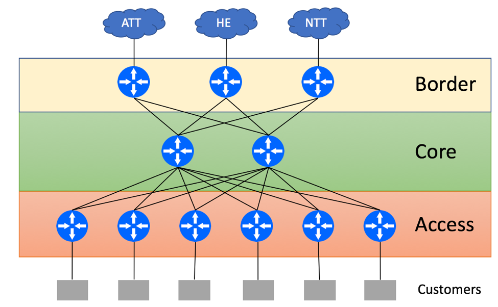
Consider the following typical Service Provider topology:
ISP Environment – Typical Topology
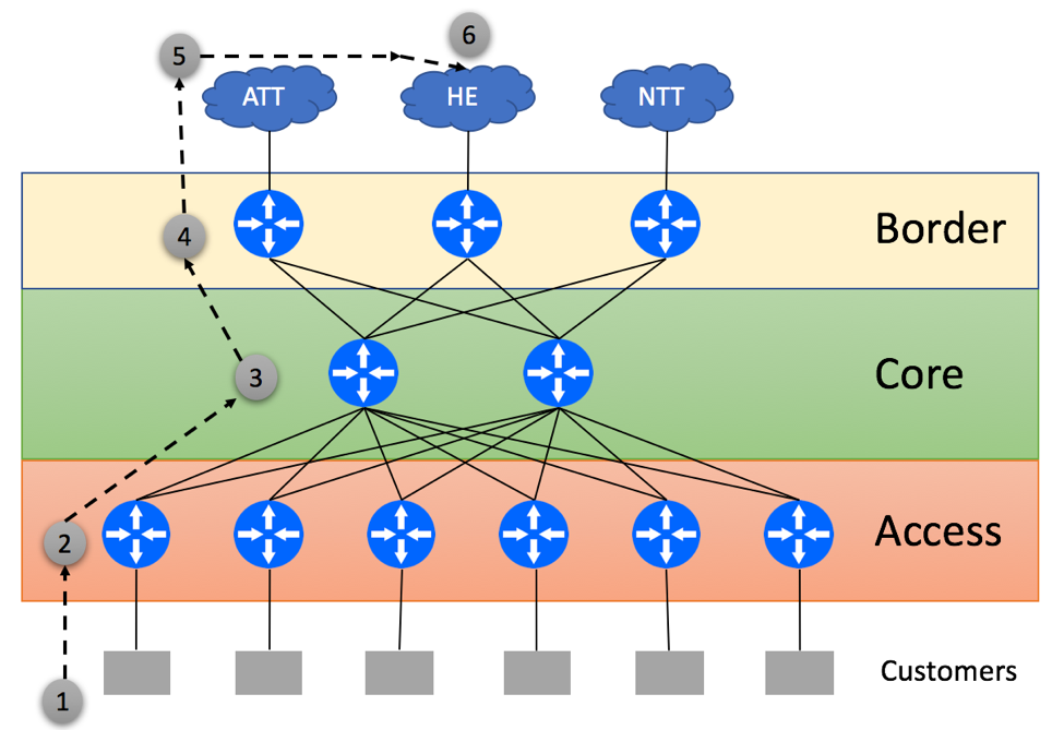
ISP has a dedicated Core Layer that aggregates connections from Border Layer devices used for external peering connectivity and Access Layer devices used for Customer connectivity. ISP is connected to three upstream providers and receives the full BGP feed from all of them. In a non-BGP-Free Core environment, Borders routers will re-advertise the routes received from external peers via IBGP to Core routers. Core routers can be used as Route-Reflectors and re-advertise full BGP view to the Access devices. If Access devices are not capable of supporting the full BGP view, you might be able to get away with advertising just the default route from the Core to Access devices. As Core routers have the full BGP view, they can find the optimal exit point for the traffic leaving the network.
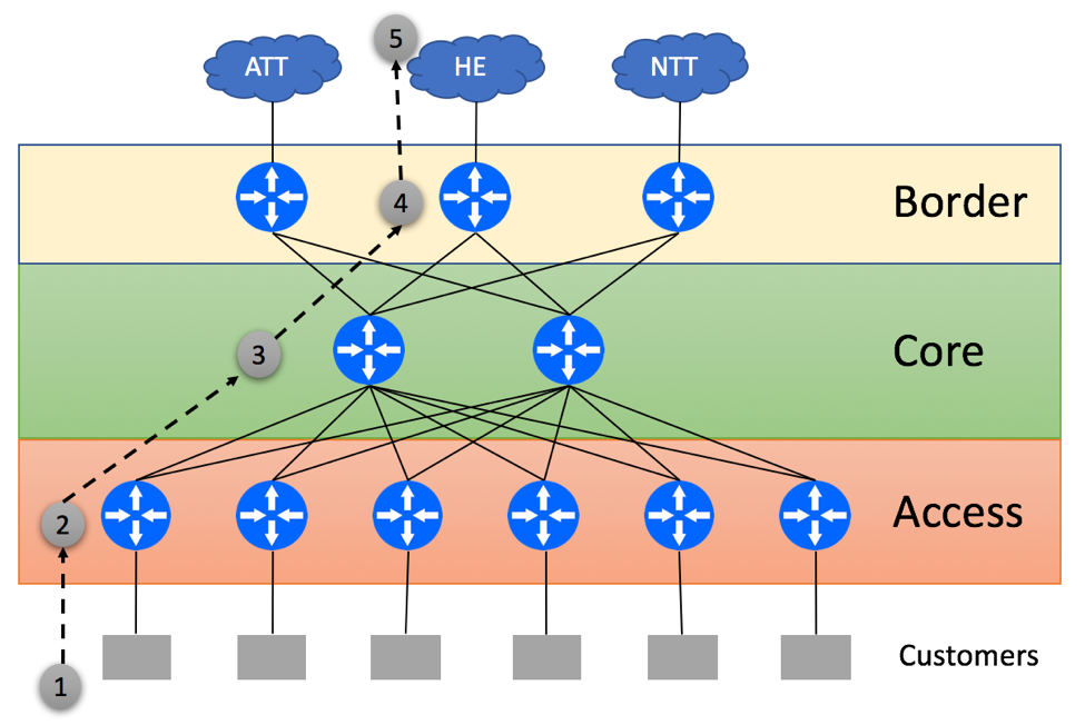
Let’s review packet flow scenario with traffic originating within ISP’s customer’s network and being destined to a prefix that resides on the HE network. In our case, ISP’s Access layer does not have the full BGP view and relies on the default route received from Core routers.
Typical Full BGP View Topology
Customer Originates the packet
Access Layer device within ISP’s network uses the default route to send packet to one of Core routers in a round-robin fashion
Core device does a lookup and determines that the destination on the HE’s network is best reachable via the middle border router
Border router forwards this packet to the HE
Server within the HE network receives the packet
Now, let’s talk about a BGP-Free Core. It is assumed that the Core has no knowledge of Customer-owned or Peer-advertised destinations and is only capable of forwarding traffic to IP destinations that belong to ISP’s internal infrastructure. Access and Border devices will have a full mesh of Tunnels (LSP’s in MPLS terminology) and will pass traffic via those tunnels.
We’ll start with the scenario where Access routers have enough RIB and FIB capacity to support the full BGP view from the Border devices.
In this case, Access layer will make optimal forwarding decisions as shown below:
Optimal Routing due to Full BGP View
Customer Originates the packet
Access Layer device does a lookup in its BGP tables and determines that the Middle Border router is the best gateway to reach the HE. Access Layer device will encapsulate customer-originated traffic into a tunnel and send it to the Border via one of the Core routers
Core device receives tunneled traffic and delivers it to the intended Border router
Middle Border Router sends packet to the HE
Server within the HE network receives the packet
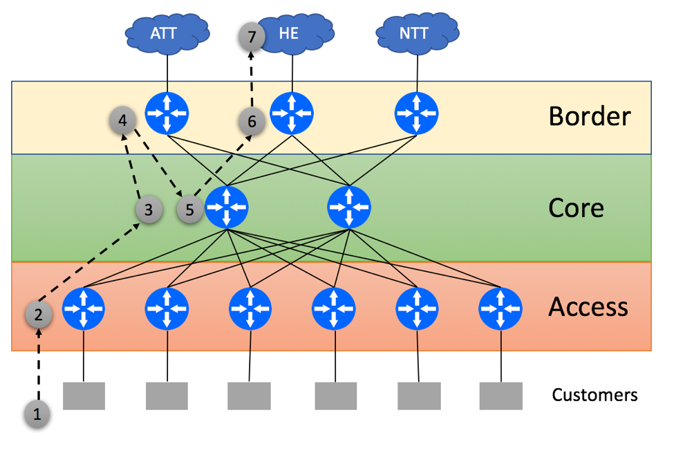
In our next scenario, Access routers are not capable of supporting the full BGP view and have to rely on the default routes, this time advertised by the Border Routers. This might lead to suboptimal traffic flow as shown below:
Suboptimal Routing due to Default-Only Routing
Customer Originates the packet
Access Layer device within ISP’s network uses the default route and tunnels packet to one of the Border routers in a round-robin fashion. It is not able to determine the best egress point, as Access device does not maintain the full BGP view
Core device tunnels the traffic to the Border device selected by the Access Layer
Left Border router does IP Destination lookup and determines that the optimal path to the prefix on the HE network is via the Middle Border. It Tunnels traffic to that Border
Core router receives a tunnel-encapsulated packet and sends it to the Middle Border
Middle Border Router sends the packet to the HE
Server within the HE network receives the packet
Another permutation of the previous scenario is shown below. This time BGP policies on the Border routers force traffic to leave via directly connected EBGP peer, even if the better path exists:
Suboptimal Routing due to BGP-Free Core and Default-Only Access
Customer Originates the packet
Access Layer device within ISP’s network uses the default route and tunnels packet to one of the Border routers in a round-robin fashion. It is not able to determine the best egress point, as Access device does not maintain the full BGP view
Core device tunnels the traffic to the Border device selected by the Access Layer
Left Border router does IP Destination lookup and selects directly connected EBGP Upstream to send the traffic
AT&T’s network delivers the packet to HE
Server within the HE network receives the packet
While both deployment scenarios allow for the traffic to be delivered to intended destinations, it is easy to spot that packets might need to traverse the additional hops. This will often lead to increased round-trip latency and unnecessary link utilization.
Conclusion
BGP-Free Core is a popular deployment mechanism that is employed by thousands of ISPs around the globe. It helps to save cost and improves operational stability of the network. With this being said, you should be aware of the deployment caveats highlighted above and be ready to address those in your network design.
BGP High Availability and Multihoming scenarios for Enterprise customers. Single ISP and Multi-ISP Redundancy.
Introduction
In this article, we will focus on building reliable Internet access to Enterprise branches. We will discuss single- and multi-homing scenarios and how BGP protocol can be leveraged in these deployments. While IPv4-based examples will be provided, this paper is also applicable to IPv6 deployment scenarios. The focus of this paper is Internet connectivity, although discussed techniques can be used for other types of connectivity, such as private IP VPN.
Enterprise BGP Internet Connectivity Options
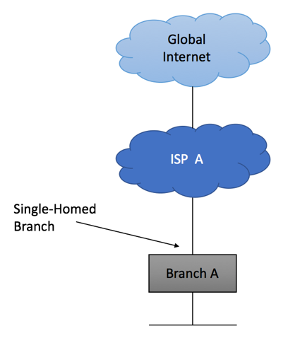
Single-homed network
As the name suggests, single-homed network is the network with just one external link. This is the type of Internet connectivity you have at home and the most common implementation scenario for small branch locations. It is simple, inexpensive and readily available. Your service provider might allocate a single IP address to the branch, requiring you to do NAT on border device, or might give you a large block allowing to assign Internet-reachable IP addresses to all branch devices.
Single Homed Site
If you were allocated only one IP address that is configured on ISP-facing interface of your border router, all you need to
Setup default route pointing towards ISP’s network
Select RFC1918 prefix that will be used to address your LAN infrastructure
Configure NAT
If ISP did provide you with a large Internet-routable block, you should come to an agreement on how this block will be advertised to the Internet.
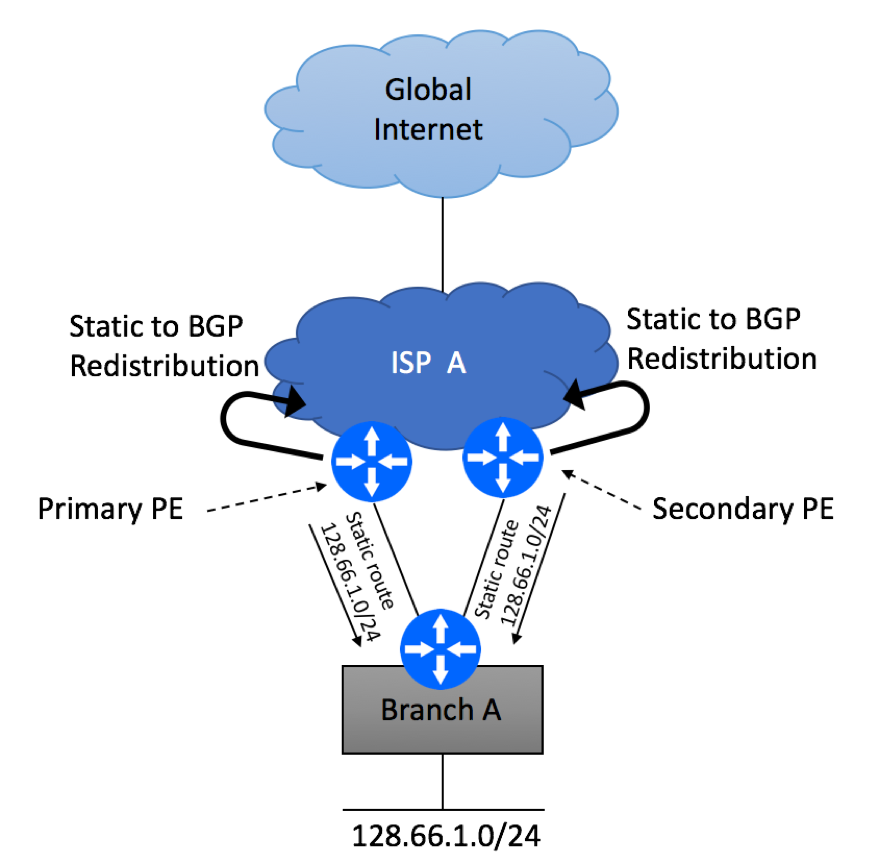
The most common scenario is the static configuration on ISP’s edge router to point to your device. For example, branch A was assigned 128.66.1.0/24 prefix.
ISP will do two things:
Configure Static Route for 128.66.1.0/24 pointing to your Customer Premises Equipment (CPE) router
Redistribute this static route into one of dynamic routing protocols, making the rest of ISP A’s infrastructure aware of the network that was assigned to you
On your end, you will configure default 0.0.0.0/0 route to point to ISP A’s router, and assign given 128.66.1.0/24 network to CPE’s branch-facing interface.
Even in a single-homed scenario, it is possible to use dynamic routing protocols to advertise 128.66.1.0/24 prefix and accept default route from the ISP, although there is no technical benefit in doing this.
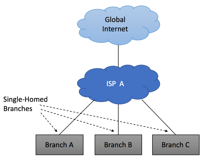
As your company grows, you might have additional offices to connect to the Internet. If these offices are connected in a similar fashion, you will still be using “Single-Homed” implementation.
Single Homed Multiple Sites
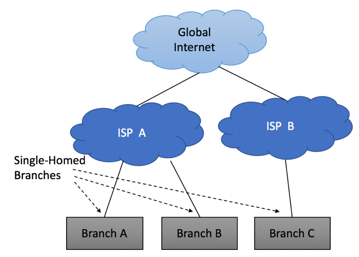
It is not uncommon to use different Service Providers to connect different branches, yet all your connections will still be “Single-Homed.”
Single Homed Multiple Sites
Multi-Homing Overview
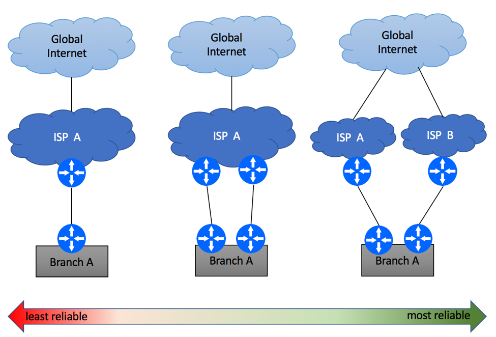
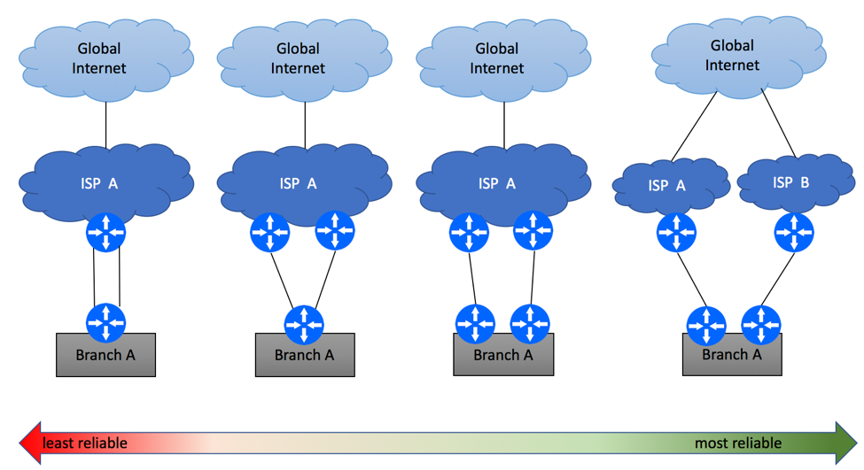
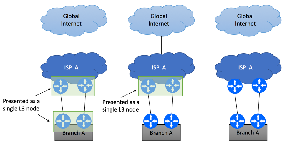
Assuming Internet connectivity is critical to your business, having a single link between ISP and your offices is a recipe for disaster. Equipment failure, fiber cuts, maintenance windows and DDoS attacks are common sources of Internet outages. In order to protect yourself, you should consider Internet multi-homing, where your branches will have an alternate path to the Internet in case of the primary link failure. While many Service Providers will be happy to sell you “redundant” Internet connectivity, it is important to understand that there are many levels of redundancy. Diagram below shows some examples, starting with the least reliable option of the secondary circuit being terminated on the same routers, and all the way to dual-homing scenario where your branch is connected to two ISP’s via two fully redundant paths.
Enterprise Multi Homing Scenarios
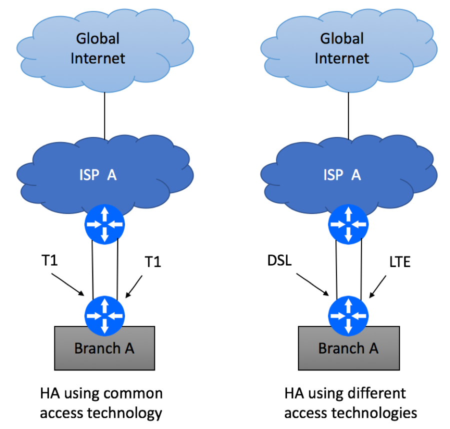
Multi-Homing Scenario 1 – Same PE / CE
The simplest and the least reliable multi-homing scenario is where two physical links are terminated on the same Layer 3 devices on both ends. Depending on ISP’s capabilities, this service might be delivered over the same (e.g. two T1 circuits) or different access (e.g. DSL and LTE) media technologies. While it is recommended to avoid this type of setups if high availability is your primary concern, this might be the only option in some geographical areas.
Multi Homed Single PE/CE
Branch device configuration will be dictated by ISP’s service offerings and might include the following options
For common access technology, ISP might offer transport bonding, where one L3 paths is created from multiple physical links. This might be called T1 bonding, Ethernet Port Channel, Ethernet Link Aggregation, etc.
In case of dissimilar technologies, two L3 paths will be created. Most commonly, these two paths will be configured in Active / Standby mode, where the primary path takes all the traffic until it is declared unusable. Then the traffic will switch over to the secondary path. Failure detection mechanisms will vary from ISP to ISP and might include L2 OAM, BFD, L3 routing.
While BGP protocol can be used for failure detection and load-balancing in single PE / single CE scenario, it provides limited benefit to you as the end user.
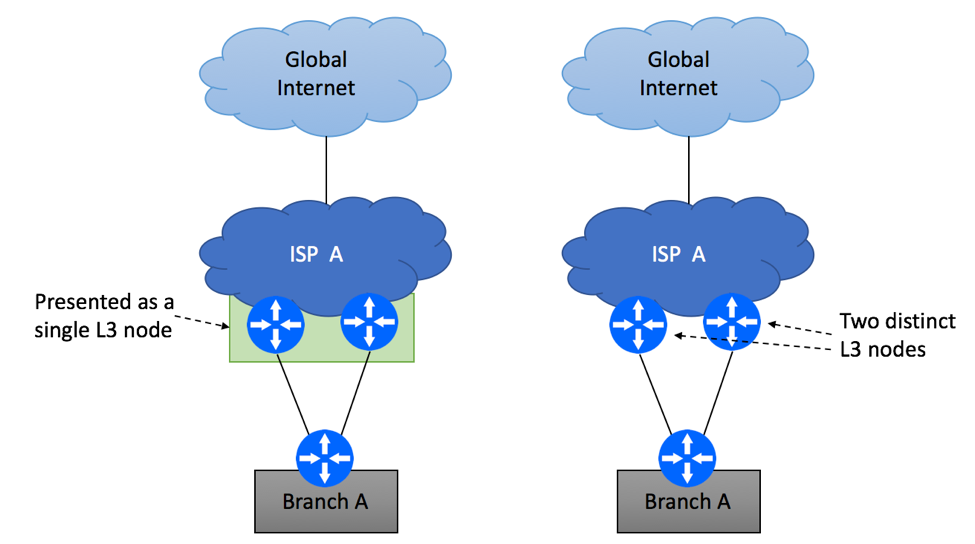
Multi-Homing Scenario 2 – Different PEs / Single CE
The second common scenario is the one where branch’s Internet circuits are terminated on two PE devices as shown below, while you continue to utilize single device at the branch site.
Multi Homed Dual PE Single CE
Your ISP might have the capability to join two physical devices into a single logical L3 node, meaning that the rest of the network (including CPE at your site) will see this combined system as a single router. The obvious benefit of this type of technology is improved availability of the service, as failure of one node will not cause an outage for dual-homed customers. There are also some known drawbacks, for example software bug or configuration mistake is likely to impact both ISP’s nodes at the same time.
The second scenario is the one where two PE devices are completely independent of each other. Most likely, this will mean that one of the physical paths will be designated as “primary” and the second as “secondary.” Both static routing and BGP are commonly used for these deployments, so let’s review both cases.
If you opt out to use static routing, ISP will configure static routes on their primary and secondary PE devices pointing to your CPE as shown below. They will then redistribute these routes into their routing protocol of choice, such as IBGP.
Multi Homed Dual PE Single CE Static Routing
ISP will also need to make sure that there is a reliable mechanism in place to detect link failure condition between your branch CPE and PE router. BFD is a popular option, although not all platforms can support it.
On the CPE side, you’ll need to configure two static routes pointing to the primary and the secondary PE devices. You have a choice of configuring these two routes with the same metric (admin distance in Cisco’s terms) or different metrics. If both of your paths have the same characteristics (bandwidth and latency), configuring equal metrics is a viable option. If your paths are not the same, for example 10Mb Ethernet as primary and T1 as secondary, configuring the primary one with lower metric and the secondary one with higher metric would make more sense.
If you decide to use BGP instead of the static routing, you’ll need to do a few things:
Request Private BGP Autonomous System (AS) Number from your ISP, unless you have a public AS assigned to you by the Regional Internet Registry
Find out what BGP AS is being used by your Service Provider
Agree on MD5 keys to use for your EBGP sessions
Ask your ISP to advertise default-route only. There is no need for you to get the full BGP view, too many routes might overwhelm your CPE device.
Ask what communities are supported by your ISP to identify the primary and the secondary paths
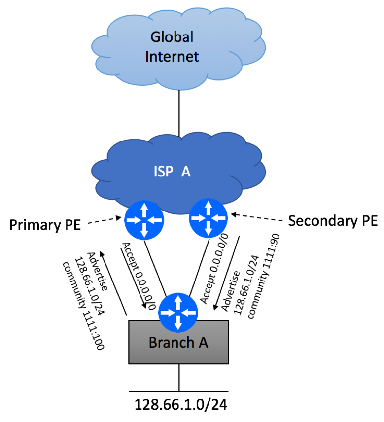
Advertise the prefix that was assigned to you with corresponding communities
Let’s assume that your ISP supports the following communities:
1111:100 – primary Internet path
1111:90 – secondary Internet path
Configure BGP sessions as shown below. Make sure you only advertise the prefix assigned to you by the ISP and not your internal routes.
Multi Homed Dual PE Single CE BGP Routing
Multi-Homing Scenario 3 – Different PEs and CEs
The third scenario requires physical router redundancy on both Service Provider’s and Customer’s sites. There are a few deployment options to be considered.
Analogous to how Service Provider might combine two physical nodes to work as a single L3 device, you can employ similar technique on your end. This can be done by leveraging proprietary vendor implementations, such as Virtual Switching Systems, Virtual Chassis, firewall clusters, etc. If you take this route, you will effectively create a single L3 node, so configuration techniques discussed in “Scenario 2” section would be applicable to this use case.
Multi Homed Dual PE Dual CE Options
If two CPE’s are not combined, you will need to rely on routing protocols to forward traffic to and from the Internet. Both static routing and BGP can still be used in a dual-CPE deployment. Let’s discuss static routing deployment first.
With static routing, your Service Provider will configure static routing and routing redistribution the same way they’d have configured it in a single-CPE scenario, but configuration of the CPE device at the customer site will be more complex.
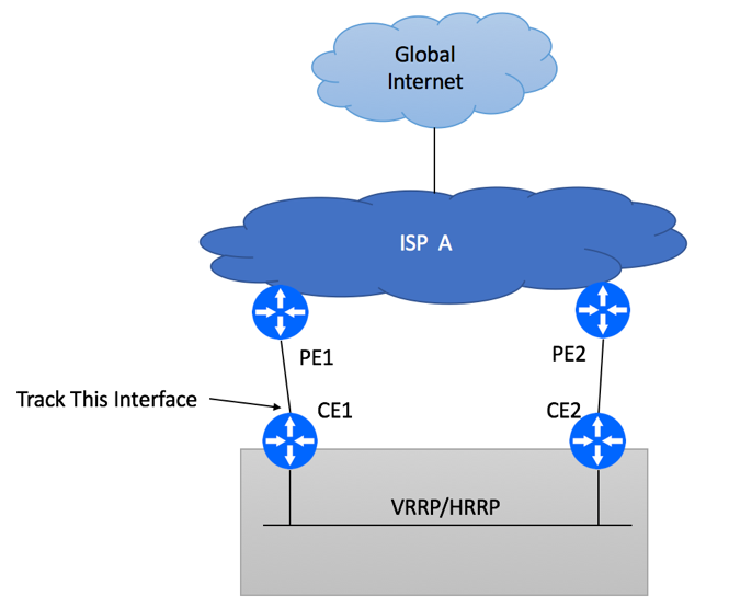
Multi Homed Dual PE Dual CE Options with HSRP/VRRP
On both CE1 and CE2 devices, configure static default routes pointing to corresponding PE devices
Decide which CPE device will be used as the primary router for Internet connectivity
Configure either VRRP or HSRP between your CPE devices. Primary device should have higher VRRP/HSRP priority. Allow pre-emption.
Configure upstream interface tracking and VRRP/HSRP priority change on upstream link failure.
As an additional protection mechanism, consider enabling IP SLA to monitor the status of ISP’s PE device modifying HSRP/VRRP priority if the device becomes unreachable. This helps to avoid blackholing if CE1 is unable to detect link failure or if PE1 experiences issues while keeping interfaces in “up” state.
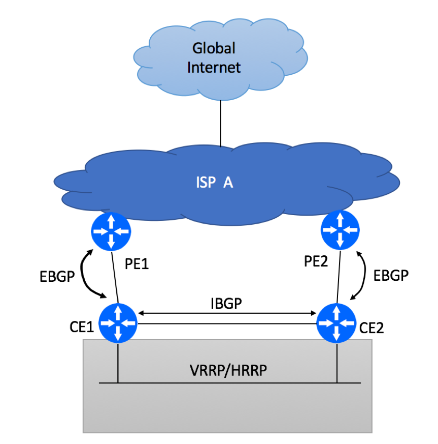
While static routing configuration might be preferred by some network administrators in dual-PE / dual-CPE deployment due to its simplicity, BGP-based configuration is a valid and in many cases preferred alternative.
Multi Homed Dual PE Dual CE Options with HSRP/VRRP and BGP
To get BGP going, follow these configuration steps:
Request Private BGP Autonomous System (AS) Number from your ISP, unless you have a public AS assigned to you by the Regional Internet Registry. You will only need one AS Number as both CE devices belong to the same site.
Find out what public AS is being used by your Service Provider
Agree on MD5 keys to use, this will secure your EBGP session
Ask your ISP to advertise default-route only. There is no need for you to get the full BGP view
Ask what communities are supported by your ISP to identify the primary and the secondary paths
Advertise the prefix that was assigned to you with corresponding communities via EBGP session
Configure IBGP session between CE devices. The purpose of this IBGP session is to exchange the default route learned from the ISP between CE devices. Under normal conditions, this IBGP-learned route will not be used as EBGP path will be preferred. But IBGP-learned prefix will get utilized when CE-PE link failure.
Configure VRRP between CE devices.
Configure upstream interface tracking and VRRP/HSRP priority change on upstream link failure. Although with IBGP session in place, you will not experience traffic blackholing, VRRP failover will help you to bypass CE router with failed upstream link.
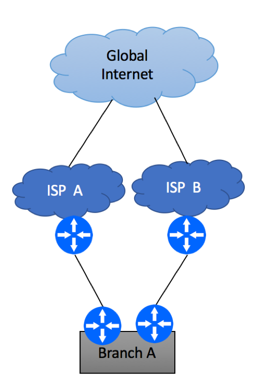
Multi-Homing Scenario 4 – Multiple ISPs
The last and the most reliable multi-homing scenario is the one where your network is connected to different service providers. As always, there are multiple flavors of this implementation.
Multihoming to different ISPs
But before we go into implementation details, ask yourself these questions:
Are there any services hosted within your branch location that need to be reachable via the Internet? An example of these services can be VPN concentrator, Web, Mail or File Server.
Can those services support multiple external IP addresses and take care of seamless failover if public IP changes? For example, Email server can be assigned two public IP addresses – one provided by the ISP A and the second IP provided by ISP B. Two DNS MX records pointing to these IP addresses will take care of the service failover. Other services, such as Web server, while capable of being reachable via multiple external IPs, will not perform well if one of the IP addresses goes away. DNS records will need to be updated to purge no longer reachable IP address, sessions in progress will drop and user experience will suffer.
Can non-graceful failover be tolerated for inside-out connectivity (users in the branch trying to reach the Internet)? Is it acceptable if all user’s session will drop and users will need to reconnect to the resources they’ve used on the Internet?
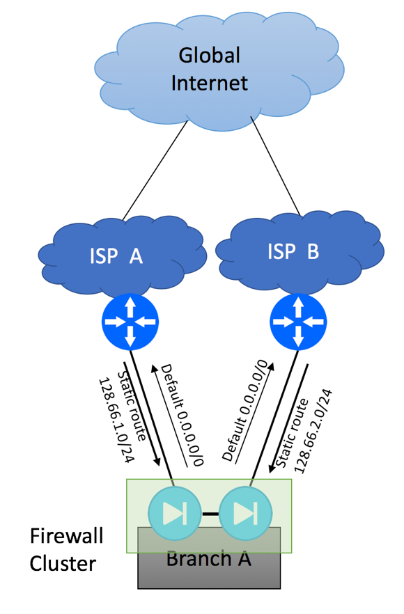
If your users can accept short period of service interruption when traffic fails over from one ISP to another, and you are not hosting any mission critical Internet-facing services in your branch location, you have a simpler problem to solve. This is nothing but a single-homed network scenario we described at the very beginning of this article, repeated twice. Your service providers will allocate IP Prefixes from their respective routable IP pools, and you will have two independent IP ranges to assign to the end devices at your branch site. Most network administrators would setup a firewall cluster and configure NAT pools using IP addresses provided by the ISPs for NAT pools. As you will be configuring two default routes on your firewall cluster pointing to two different Service Providers, there will be a need to implement policy-based routing on your device to make sure traffic with a wrong source IP is not being sent. For example, you got 128.66.1.0/24 allocation from ISP A and 128.66.2.0/24 from ISP B.
Multihoming to different ISPs with Firewall Cluster
Please note that you should never try to send packets with source IP in 128.66.1.0/24 range to ISP B and packets with source IP 128.66.2.0/24 to ISP A, as ISP’s anti-spoofing mechanisms such as uRPF might drop these packets. Your policy-based routing configuration should check the source IP of the packet and send it via correct egress interface.
If the services hosted in your branch location require 100% uptime and cannot allow external IP change, you must implement BGP. You’ll need to follow the steps outlined below:
Make sure your Internet providers can support BGP over your transport media. For example, some ISPs will allow you to run BGP over T1 and Ethernet-based links but not over DSL and 3G and LTE.
Request Public Autonomous System (AS) number from one of the Regional Internet Registries (ARIN, RIPE, APNIC, LACNIC or AFRINIC). In order to qualify for AS, you will need to meet the following requirements: “If you are qualifying under the multihomed policy you will need to provide the exterior gateway protocol to be used, the IP addresses currently in use on your network, the AS number and name of each of your upstream providers and/or peers along with contractual verification of service with at least two of them.” Source: http://teamarin.net/2014/01/31/how-to-request-an-asn-from-arin/
Request publicly-routable IP prefix. This might become the most difficult part of your project. Due to IPv4 depletion, it is very unlikely that you will be able to get direct allocation from one of the RIRs. This means that you will need to get routable IPv4 space from one of your ISPs, and get their permission to start BGP advertisement of this space from your own AS via a different ISP!
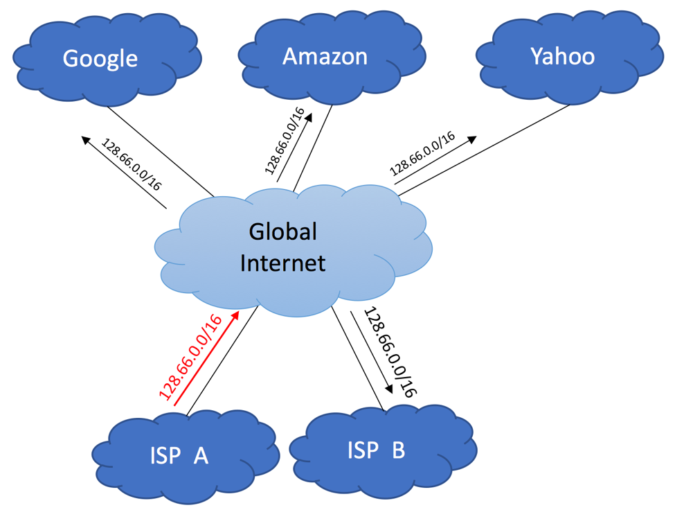
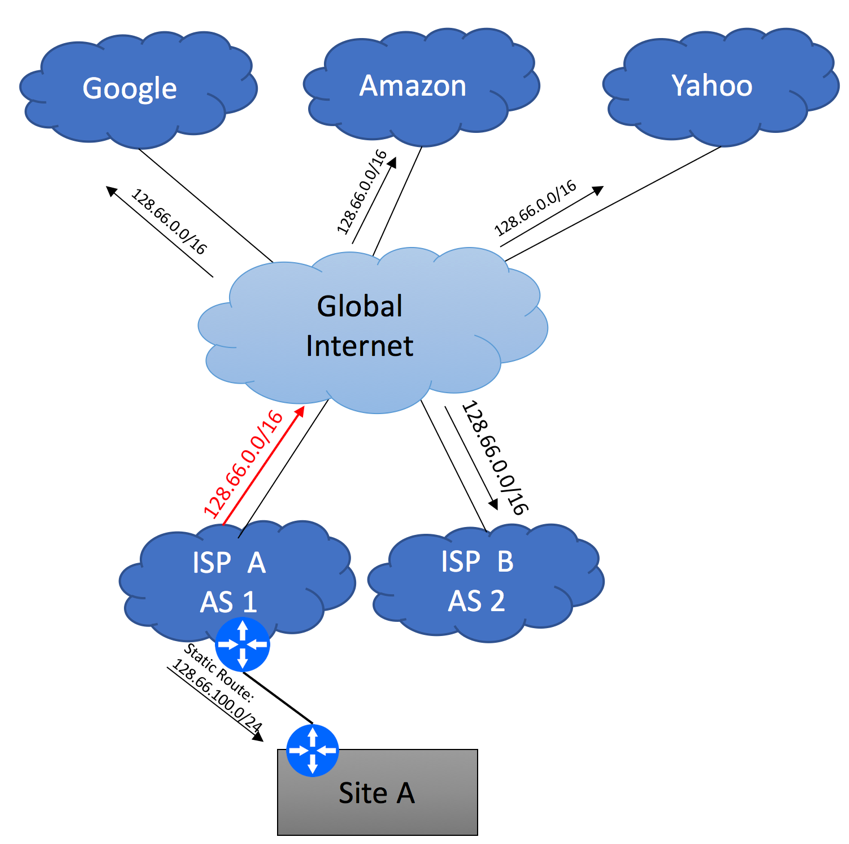
Here is an example to illustrate this scenario. Imagine, that ISP A was assigned 128.66.0.0/16 by RIPE. Being a good Internet citizen, ISP A advertises this aggregate block via BGP to the Internet, while suppressing smaller advertisements.
Multihoming to different ISPs using BGP
ISP B receives this advertisement as a part of the Global Routing Table update either from ISP A (assuming ISP A and ISP B maintain direct peering relationships), or via 3-rd party service provider. The same applies to all other companies that participate in the global BGP.
Now, let’s pretend that ISP A assigned 128.66.100.0/24 prefix to your Site A. Information about this 128.66.100.0/24 network would need to be propagated within ISP A’s network, so that traffic coming from the global Internet could find its way to your circuit, but specific 128.66.100.0/24 advertisement does not have to be sent to the Internet. 128.66.0.0/16 that is currently being advertised already includes 128.66.100.0/24 block, making it reachable from everywhere. More specific 128.66.100.0/24 advertisement originated from your Site A will be suppressed by ISP A and will not be leaked to the Global Internet.
Multihoming to different ISPs using BGP
It is not important if ISP A uses static routing between their PE device or rely on BGP – in order to be good internet citizens, they should suppress 128.66.100.0/24 advertisement.
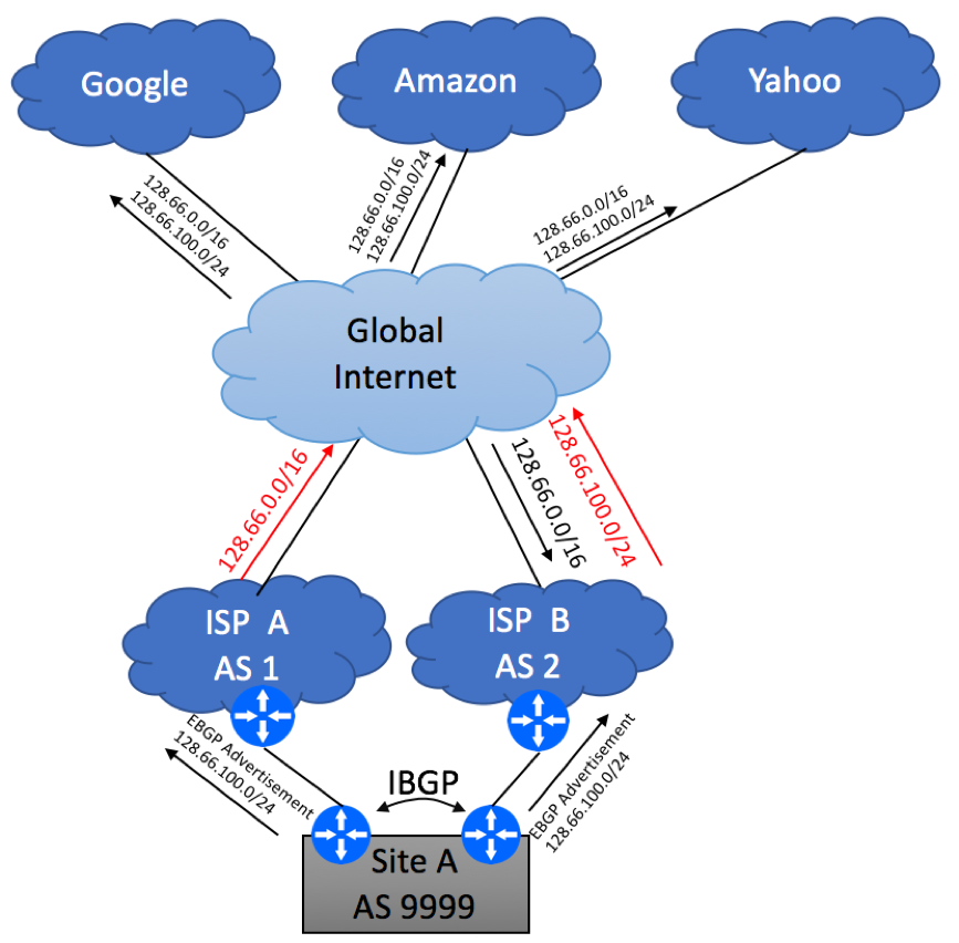
As your end goal is to start advertising 128.66.100.0/24 from your own AS, let’s review the following example, assuming that ISP A’s public AS number is 1, ISP B’s Public AS number is 2 and your company got assigned AS 9999.
In the initial state, when ISP A receives 128.66.100.0/24 advertisement originated from AS 9999 they will not propagate it to the Global Internet. This is perfectly fine, as the only way for the Internet to reach Site A is via ISP A, and ISP A already originates an aggregate 128.66.0.0/16 block. By sending your 128.66.100.0/24 to the rest of the Internet, ISP A will increase the size of Global BGP table for everybody without achieving any benefits.
Multihoming to different ISPs using BGP
Your next step is to establish EBGP peering between Site A and ISP B and advertise 128.66.100.0/24 to ISP B. You will need to get an approval from ISP A for this, and you will need to present this approval to ISP B.
As ISP B does not own 128.66.100.0/24 or any part of 128.66.0.0/16, there is no way for the to aggregate /24 prefix, so they will re-advertise your 128.66.100.0/24 prefix to the rest of the Internet. Now we observe an interesting paradox, where the global Internet starts using ISP B to send traffic to your Site A, despite the fact that 128.66.100.0/24 prefix is owned by ISP A. You can attempt to do AS prepend on your advertisements towards ISP B, but it will not make a difference, as more specific route will always win. The only traffic you might observe on your ISP A – Site A link is the traffic originated from ISP A’s direct clients.
Multihoming to different ISPs using BGP
If redundancy is your only concern and ISP A is fine with the fact that the majority of your traffic is being sent via their competitor, you can stop here. Failover will work as it is. If your CE2 or CE2 to ISP B’s link goes down, or even if the entire ISP B disappears, traffic will get rerouted via ISP A thanks to the aggregate 128.66.0.0/16 block being advertised by ISP A.
If this situation is not acceptable and you due to load-balancing requirements or ISP A insists on seeing CE1 – ISP A being used under normal conditions, ISP A will have no choice but to stop suppressing your specific advertisement and start leaking 128.66.100.0/24 originated from AS 9999 to their peers. This will take care of the traffic coming to the Internet and destined to your network. It is not possible to say ahead of time what percentage of the incoming traffic will come via ISP A vs ISP B, but there will be some level of load balancing.
The next step is to figure out the best way to send the traffic from your site to the Internet. The simplest solution is to accept the default 0.0.0.0/0 route from both ISP A and ISP B. If you have a preference for the primary path, you can configure ingress BGP policy and set higher BGP local preference for the default route coming from either ISP A or ISP B. If your routers are capable of supporting the full BGP view (meaning they can handle close to 1Mln routes), you can request your ISPs to send you the full Internet routing table. Leave it to BGP to decide what path to take to reach the Internet destinations. And don’t forget to configure IBGP session between your CE devices!
In this article, we will discuss various types of Internet peering. You need to have basic knowledge of BGP protocol to better understand this paper, so if you are not familiar with BGP, we suggest that you start with the following Wikipedia article: https://en.wikipedia.org/wiki/Border_Gateway_Protocol
As a peering administrator, you are responsible for selecting the best peering strategy for your company. In order to determine what’s best for your organization, you need to identify your peering goals. Very frequently, these goals might be at odds. Let’s start with reviewing possible peering objectives and then continue with a discussion on why it is difficult to satisfy all of these requirements at the same time.
Typical Service Provider would have the following peering objectives:
Achieve High Availability – no matter what happens, your network should be able to reach any Internet destination
Maintain Low Latency and Low Packet Loss – you should always try to pick the path with the lowest possible latency and minimum packet loss
Minimize Traffic Cost – achieve the best connectivity possible at the minimal cost possible
Maximize Revenue – this often means that you want to attract more customers’ traffic than your competitors
By going through the objectives list, it is clear that the low-cost goal is at odds with other stated objectives. To achieve the best connectivity and high availability, you’d need to peer with as many companies as possible, but peering costs money. At the same time, improved peering might lead to increased revenue, as your network will attract more traffic.
The reality of the situation is that you will need to find a compromise by determining the number and types of peering that is right for your company.
Let’s list the types of peering sessions and then reveal technical details associated with each of them:
Upstream, also known as Transit Peering
Private Peering
Public Peering
Downstream, typically Customer Peering
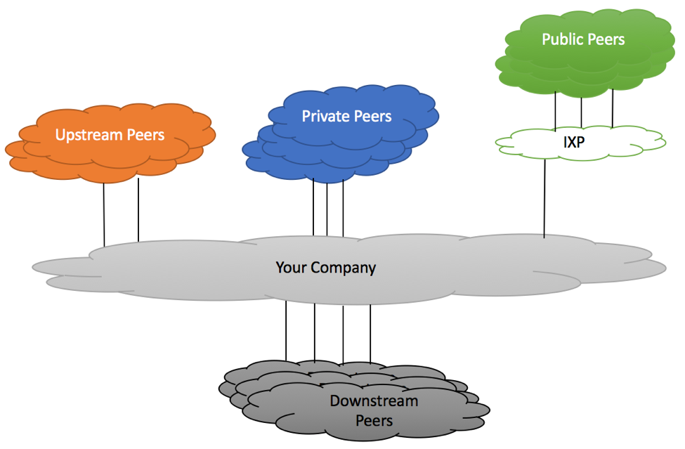
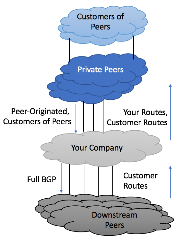
Figure below shows an ISP (labeled as “Your Company”) connected to different types of peering partners.
Types of Peering
Upstream Connectivity / Transit Providers
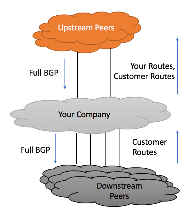
Unless you work for the elite group of Tier 1 providers (https://en.wikipedia.org/wiki/Tier_1_network) you will always need to buy Internet Transit Service from one or more service providers. This Transit Connectivity is sold by Upstream providers, who will feed you the full Internet BGP view table and, at least in theory, will deliver your packets to any device on the Internet either over their own network, or via their partners and clients. Selecting the right upstream provider or group of upstream providers is one the most important decisions you’ll need to make while building your network. Reliability, Connectivity types, cost per Mb are just some of the factors that will influence this decision. We’ll talk about selecting the right Upstream later in this article.
By accepting the full BGP table from Transit provider, your routers’ routing tables will get populated with the information about each and every IPv4 (and possibly IPv6) prefix currently present on the Internet.
In return, you will advertise your locally-originated routes, as well as routes received from your BGP customers.
Upstream / Transit Peering
Most organizations will employ direct transport links with their Transit providers, although it is possible (but typically not cost-effective) to leverage physical transport provided by an Internet Exchange Point (IXP) for upstream connectivity.
Private Peering
Private peering is the type of peering where two parties establish BGP connectivity over direct transport link and exchange information about routes originated in their own and their customers’ networks. While most of private peering arrangements are settlement-free, meaning that companies do not pay each over to exchange traffic over private links, there are also cases where an ISP might refuse to establish settlement-free relationships with your company, but is willing to sell access to their customer base at a discount, as compared to buying full transit connectivity from that provider.
It is also important to remember that while the traffic exchange might be free, there will be a cost associated with the physical transport (e.g. 10GE link over DWDM), as well as the cost of a port on your router where this link will be terminated.
In some cases, it might be difficult to predict how much traffic you will exchange with specific peer before establishing direct peering relationships. Although various traffic analysis tools such as Arbor SP might provide you with an estimate, we find that these predictions are not always reliable.
When possible, you should start with establishing Public peering relationships with a prospective peer and, assuming the amount of traffic justifies this, later convert to the Private peering relationships.
Figure below depicts private peering relationships with “Your Company”. Depending on the size of the peer, you might receive from them anywhere from a few routes to tens of thousands of routes. Large number of routes does not necessary mean high volume of traffic. Big CDN provider with just a few prefixes can deliver much more traffic to your network, than an ISP with thousands of prefixes in some remote geography.
Private Peering
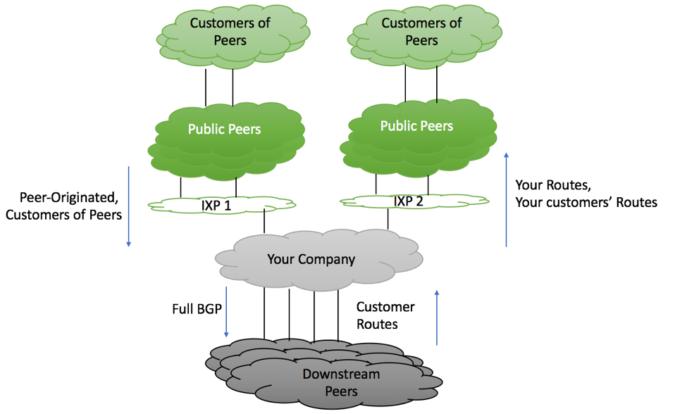
Public Peering
Public peering is a type of relationship where two companies exchange IP traffic via one of public Internet Exchange Peering Points (IXP). The main advantage of peering at IXP is the ability to establish sessions with a large number (often hundreds) of partners, without the need to build individual transport links with all these peers. While most of peering relationships at IXP’s are settlement-free, there is often an initial connectivity cost, as well as a monthly recurring cost charged for IXP connectivity. In addition to that, there is a cost associated with a transport link between your peering router and IXP port. In fact, IXP charge and the transport cost when added together, might exceed the cost of buying IP transport from one of the Transit Providers.
Public Peering
With this being said, it is always good to be aware of the peering options in your geography, as not being connected to large IXPs might put you at a competitive disadvantage.
List of Internet exchange points by size can be found here:
It is also important to note, that presence at an IXP does not automatically mean that you will be able to peer with all Exchange members. While some IXP participants have open peering policy, meaning they will exchange traffic with any other IXP member, other organizations are more restrictive and you will need to negotiate peering relationships with them on a case-by-case basis.
Downstream (Customer) Peering
BGP peering with your customers, also known as Downstream peering, is the type of a relationship where your company performs the function of a Transit Provider. IP Prefixes received from downstream peers should be re-advertised to all your peers, including Public, Private, Transit, as well as your other BGP-speaking customers.
Now that you’ve been introduced to various types of peering, let us review a few use cases.
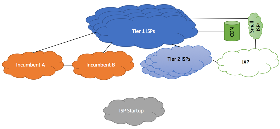
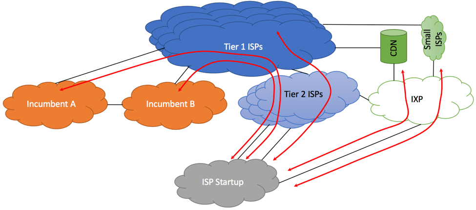
Case Study – Small ISP Startup
You were asked to recommend a peering and transit policy for a small regional Internet provider called “ISP Startup.” This company operates in the country where two large incumbent providers control nearly 80% of the country’s user base. These incumbents buy transit connectivity from various Tier 1 ISPs. Incumbents peer with each other, but will not join settlement-free peering relationships with small local ISPs.
There is an Internet Exchange point in the country. Some Global Content Delivery Networks (CDN), small local ISPs and Enterprises are connected to this IXP.
At the moment, “ISP Startup” does not have any BGP clients, but plans to acquire them in the future. The current goal is to minimize the Internet transit cost, while providing the best possible service to end users.
Based on the information provided, our “ISP Startup” has the following connectivity options to consider:
Buy transit from “Incumbent A”
Buy transit from “Incumbent B”
Buy transit from Global Tier 1 providers used by one or both Incumbent ISPs
Buy transit from Global Tier 1 providers not used by Incumbent ISPs
Buy transit from Global Tier 2 / Tier 3 providers operating in the country
Connect to Internet Exchange Point and try to establish settlement-free sessions
Figure below depicts connectivity alternatives for the new ISP.
Small ISP Peering
This use case will not be complete without some assumptions about transit costs.
Let’s use the following model:
Option
Price per Gb/month
Remarks
Incumbent A
$200
Incumbent B
$250
Tier 1 – A
$180
Tier 1 – B
$220
Used by Incumbents
Tier 1 – C
$300
Tier 2 – A
$140
Tier 2 – B
$160
IXP
$50
Will not provide transit
IXP is the cheapest option by far, but it is not a substitute for Transit Internet connectivity. It might be relatively inexpensive to connect to an IXP, but our “ISP Startup” may be disappointed by the amount of traffic exchanged over IXP links. While there are many contributing factors (a type of ISP’s own customer base, number and type of IXP participants), you should not expect to offload more than 30% of your traffic to IXP. In fact, this number might be significantly lower than that. Your next decision is to select one or more upstream providers. If you base your decision on cost, “Tier 2 – A” ISP is the winner. You would establish at least two redundant links to “Tier 2 – A”, and might build a non-redundant link to the IXP as shown below.
Small ISP – Single Upstream
Various traffic flow scenarios under normal conditions are depicted below:
Small ISP – Single Upstream Traffic Flow
While this design allows you to keep the cost low, it has a few major shortcomings:
Small ISP – Multiple Upstreams
There is no upstream redundancy – failure of “Tier 2 – A” ISP would take your company off the air.
You customers might experience high latency while communicating to Incumbent’s clients, as they’d need to cross multiple networks
If your ISP Startup grows and you acquire BGP customers of your own, it will be difficult to attract transit traffic, as your network will be a few AS hops from the majority of Internet destinations.
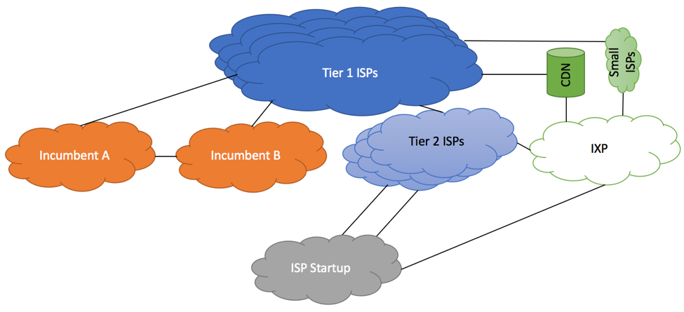
Let’s look into an alternative where ISP Startup connects to “Incumbent A”, “Tier 1 – A” and IXP.
Link to “Incumbent A” will provide you with direct access to “Incumbent A’s” customer base, as well as with a short path to “Incumbent B’s” clients. IXP connection will help you to reach the remaining local ISPs and provide access to CDN networks. Direct “Tier 1” connection will give you access to the rest of the Internet.
If Tier 1 link were to fail, you would reroute your traffic to the Internet via Incumbent A. If links to “Incumbent A” or IXP were to fail, you would reroute via “Tier 1” ISP. In addition to that, it will be much easier to attract transit internet traffic to your AS, if you peer directly with one of the global Tier 1 providers.
Let us compare monthly costs, based on the assumption that your network needs 100Gb pipe, of which 10% can be offloaded to IXP, 20% is destined to Incumbent providers and the rest needs to go to the Internet.
Option 1:
IXP: 10Gb @ $50 = $500
Tier 2 – A: 90 Gb @ $140 = $12,600
Total: $13,100 per month
Option 2:
IXP: 10Gb @ $50 = $500
Incumbent A: 20Gb @ $200 = $4,000
Tier 1 – A: 70Gb @ @180 = $12,600
Total: $17,100 per month
As you can see, Option B is ~30% more expensive. You will need to decide, if increased redundancy and improved latency warrants this premium.
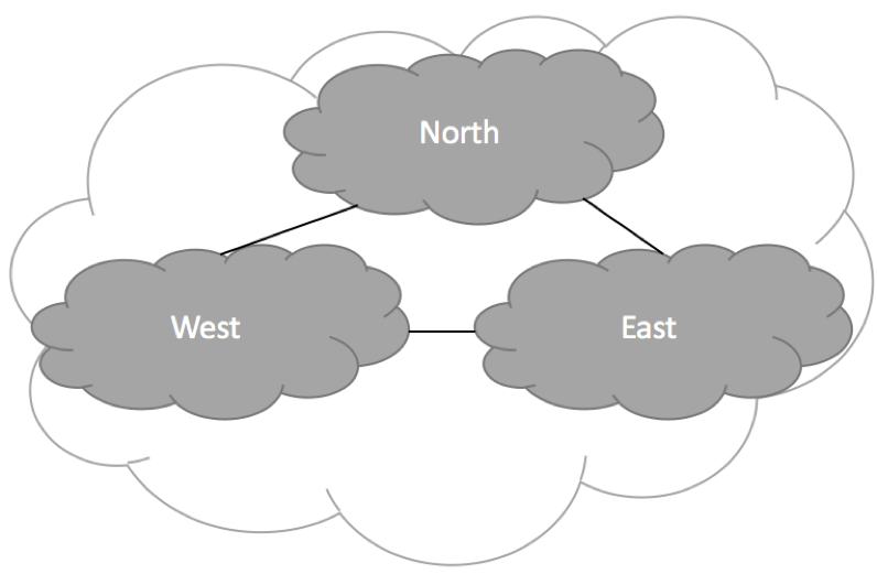
Case Study – Medium-Size ISP Operating in 3 Regions
In this case study, we will analyze the scenario of an ISP operating in 3 different geographical regions using one common AS Number. We’ll call these regions West – North – East, although in the real life they can represent three cities, countries or even continents.
Medium Size ISP
Similar to the previous example, this Medium-Size ISP needs to decide on the best connectivity options, while delivering exceptional service to its customers at the lowest possible price points.
Let’s review Transit, Public and Private peering options.
Transit Peering
Because of the size of the company and its desire to attract BGP clients, our ISP is inclined to buy transit from Tier 1 ISPs only. It believes that sometime in the future it will be in the position to negotiate settlement-free peering with Global Tier 2 providers, making it not feasible to buy transit from one of them today.
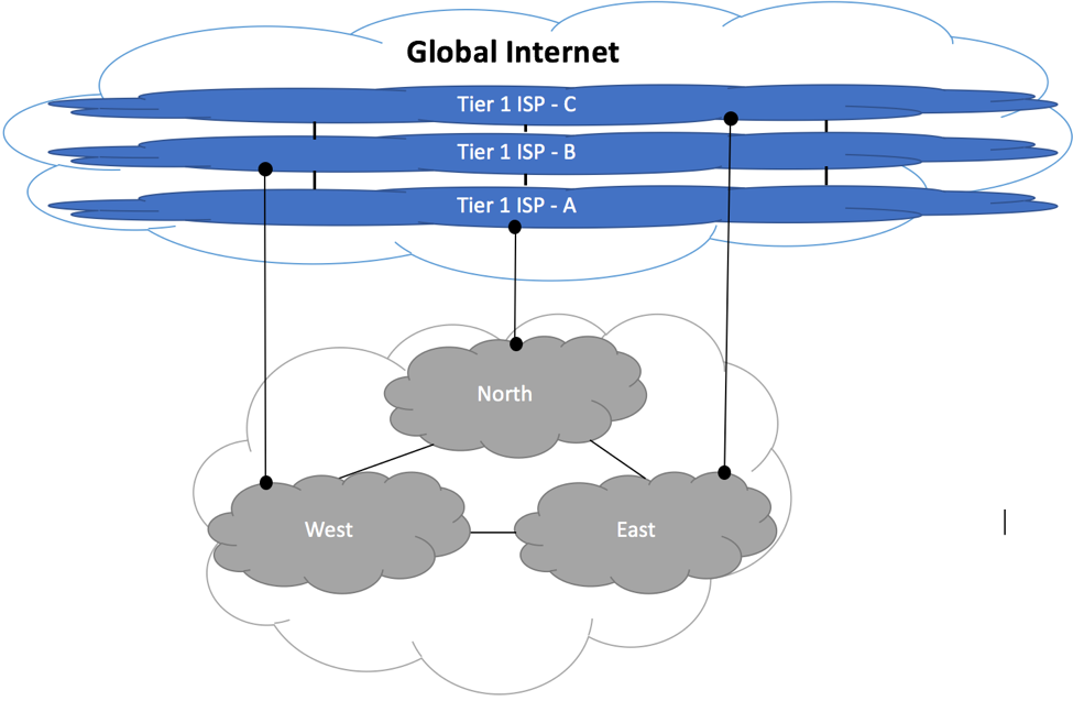
When it comes to choosing an ISP, the first possible approach is to select three different transit ISPs, one per region.
Medium Size ISP – Upstream Option 1
The clear advantage of this approach is the resiliency of Global Internet connectivity. If one, or even two links to Tier 1 ISPs were to fail, traffic could always be rerouted via the remaining connections.
It is also believed, that direct connectivity to multiple Tier 1 ISPs would help you to attract Internet traffic from your own BGP clients, making your company more profitable.
Unfortunately, while this design might look very appealing at first, there are some major drawbacks you need to consider:
You might not be able to negotiate an attractive per Mb transit rate, as your per-Tier 1 ISP traffic commitment in each of the regions will be relatively low.
Sub-optimal routing and possible high latency that you are likely to experience. Let’s explain technical reasons to why this might happen.
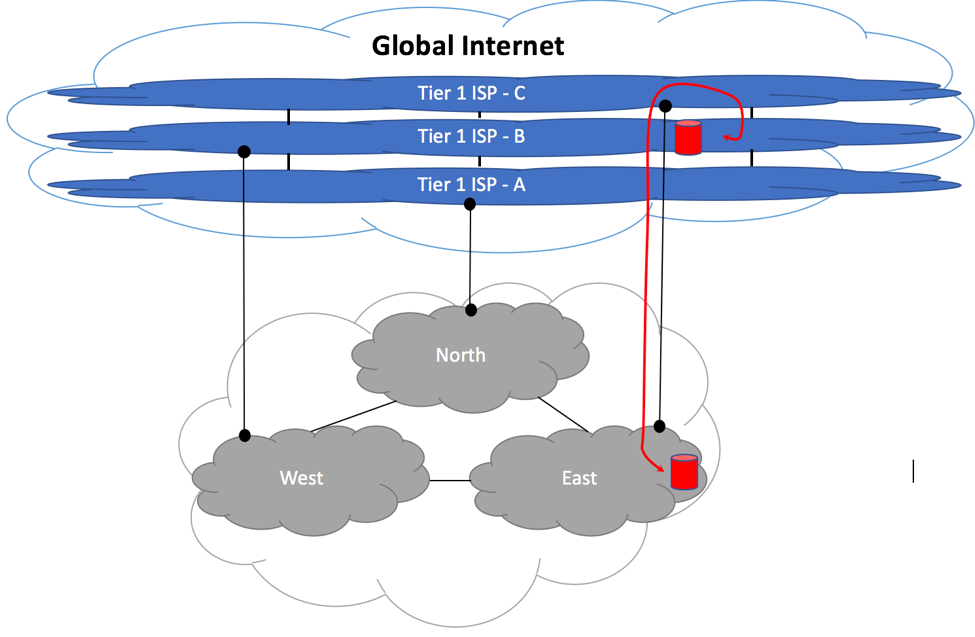
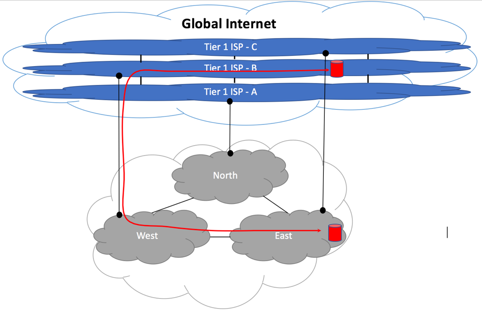
Let us consider a scenario where ISP-B’s client residing in the same geography as the “East” section of your network wants to communicate with you client. You’d achieve the lowest latency, if traffic from ISP-B would pass via ISP-C and enter your network as shown below:
Medium Size ISP – Suboptimal Upstream Peering
Unfortunately, this is unlikely to happen. For redundancy reasons, you should be advertising your “East” routes to “ISP-B” via the “West” peering point. And because the shortest AS-Path wins, default traffic flow will be as shown below:
Medium Size ISP – Suboptimal Upstream Peering
While this type of traffic flow might be acceptable, if your North / West / East regions are just a few miles away, it may pose a problem if there is a significant distance between them. Due to the speed of light limitations, distance always translates into packet latency.
You can try to manipulate your BGP advertisements towards upstream providers, setting AS-Prepend or sending BGP communities in the attempt to prevent this sub-optimal traffic flow from happening, but you are unlikely to find an acceptable remedy for this scenario. BGP protocol likes shortest AS Paths and ISPs prefer to send traffic to their directly connected clients instead of passing through a third party.
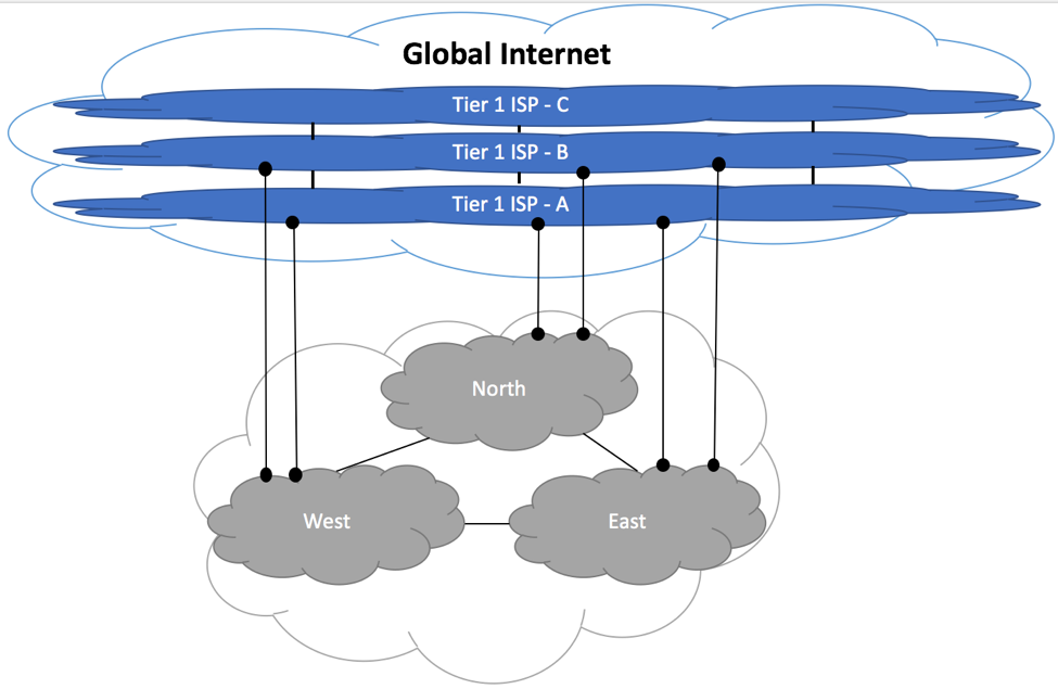
Instead of connecting to three different Service Providers across three geographical regions, you might be better off by picking just two transit providers, but connecting to both of these providers in all three geographies.
Medium Size ISP – Upstream Peering
Under normal conditions, you’d see the optimal traffic flow between the Global Internet and any of your regions. If one of the links were to fail, traffic to that ISP would reroute via two remaining links. This will increase end-to-end latency for some destinations, but this tradeoff should be acceptable.
Public Peering
As described in the “Pubic Peering” section of this paper, IXP locations are great places to establish direct connectivity to a large number of ISPs, Enterprises and CDN providers. As such, it is encouraged to be present at the public exchange points within ISP’s operating geography, and if cost permits, outside of operational boundaries. For example, service provider operating in Portugal, Spain and France should consider connecting to the largest European Peering points in Germany (DE-CIX), Amsterdam (AMX-IX) and London (LINX).
When establishing peering relationships, ISP should consider its own geography as well as peer’s geographical presence.
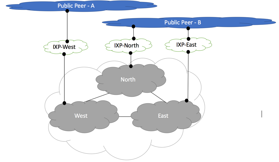
Figure below depicts potential peering scenario, where peering relationships could be established with “Public Peer – A” and “Public Peer – B”.
“Public Peer – A” operates in West and North regions, as well as some other geographies, not covered by you.
“Public Peer – B” operates in North and East regions, and also some other non-overlapping regions.
It should be no brainer to establish peering with “Public Peer – B” via “IXP-North” and “IXP-East”, as you would achieve optimal traffic flow between you two companies. Traffic originated from the West region will leverage IXP-North / IXP-East exchange points. This is acceptable as “Public Peer-B” is not present in the West.
Medium Size ISP – Upstream Peering
Decision to peer with “Public Peer – A” is more difficult. You can only peer at “IXP-West”, as “Public Peer – A” is not present at other exchange points. This will lead to sub-optimal traffic flow between your “North” customers and “Public Peer-A” customers located in the North region. You are almost guaranteed to achieve better performance by sending the North traffic via one of upstream providers. Recommended solution to this problem is to advertise a subset of your routes to “Public Peer – A”. Instead of sending all the routes originated by your company and your BGP downstream customers, only advertise the routes originated in the “West” region. The same should apply to the routes advertised by “Public Peer – A”. Request your partner to limit their advertisement to their Western routes. Use your transit provider to exchange traffic between “Peer-A” Northern region and your North and East areas.
Private Peering
Most of the service providers start their peering relationships at IXP and upon achieving certain traffic volume might later switch to a private peering arrangement. By switching to private links and bypassing IXP, they can both improve network availability and decrease traffic cost. Peering recommendations covered in Transit and Public sections of this document are also applicable to private peering arrangements. If companies operate in the same geographical regions, they should establish peering sessions in as many points as possible in order to minimize end-to-end latency.
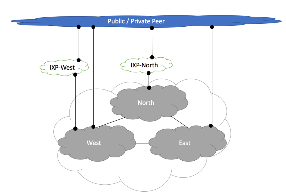
It is not uncommon to see a connectivity scenario, where two companies leverage private connectivity arrangements in some areas, while relying on public peering in other areas. Even after building direct links to a peering partner, you can still maintain BGP sessions at public peering points, diversifying your connectivity. Obviously, you’ll need to manipulate BGP attributes to make sure that private links are preferred over public exchanges. Next diagram depicts such hybrid scenario.
Medium Size ISP – Private Peering
Private peering links were established in the East and West regions. In the West region, companies decided to preserve existing public peering relationships to maintain direct connectivity in case of the private link failure. Direct peering in the North was considered unfeasible due to low traffic volume. As such, two companies rely on “IXP-North” for local traffic exchange.
One final word of caution: when it comes to private connectivity – make sure you properly size your links. It is not uncommon to run into situations where direct private peering might become harmful. Let’s illustrate this with an example:
Our Medium-size ISP has two 100GE links per region to two transit providers. There are also 10GE links to IXP-West, IXP-North, IXP-West. While peering in these locations, Company XYZ was identified as a candidate for private peering connectivity. Netflow data shows that during peak hours, 300Mb/sec of traffic is being exchanged between the two companies. As a result, it is decided to build direct 1GE links in all three geographic regions. Everything works great until Company XYZ releases a new version of their software, and many customers on the Internet decide to download it at the same time. This causes a major congestion on private 1GE links. If companies were not to switch to the private peering and leveraged 10GE IXP connections instead, they would have easily coped with this sudden traffic increase.
In this article, we will attempt to forecast the size of global internet routing table and analyze the potential impact of aforementioned routing growth on the stability of Internet infrastructure.
Global routing infrastructure is comprised of IPv4 and IPv6 routes advertised by BGP-speaking service providers and enterprises. These BGP advertisements are processed by the routers and eventually programmed into special tables called Forwarding Information Table (FIB). There is a limit a number of FIB entries a particular system can support before running out of FIB capacity. The maximum FIB capacity of the platform is determined by such factors as ASIC, amount of memory, software license, etc.
Even within a single vendor’s portfolio, the maximum FIB size of available platforms varies dramatically, from a few thousand entries in a low-cost top or rack switch up to millions of entries in an expensive Internet router. It is important to note, that advertised FIB numbers may only be applicable to certain (typically IPv4) routes. Other route types, such as MPLS VPN and IPv6, might require more memory per entry, decreasing the overall FIB capacity.
For example, Cisco’s Catalyst 6500 / 7600 with 3BXL supervisor can support 1 Million IPv4 routes, but only 512K IPv6 routes.
It is also important to note, that not all vendors will support dynamic allocation of FIB entries between route-types. Instead, FIB might be pre-partitioned to support some arbitrary number of entries of a certain type. Previously mentioned 3BXL supervisor comes preconfigured to support 512K IPv4 + MPLS entries and 256K IPv6 + Multicast entries. It is easy to spot that in Cisco’s SUP720 implementation IPv6 routes take twice as much space as IPv4 entries.
Historic perspective
The problem of FIB capacity and growing Internet size is not new.
Multiple outages were reported back in 2008 when Internet BGP table size crossed 256K limit and again in 2014 when 512K entries limit was exceeded.
Service Providers and BGP-speaking enterprises had to take remedial actions in order to maintain Internet stability. We will discuss these actions later.
Internet Growth
There are two major forces that drive Internet table size growth – IPv4 space partitioning and new IPv6 advertisements.
IPv4 address exhaustion (https://en.wikipedia.org/wiki/IPv4_address_exhaustion) that occurred before 2011 and 2015 did not slow down the speed of IPv4 table growth, instead it accelerated the fragmentation of IPv4 space.
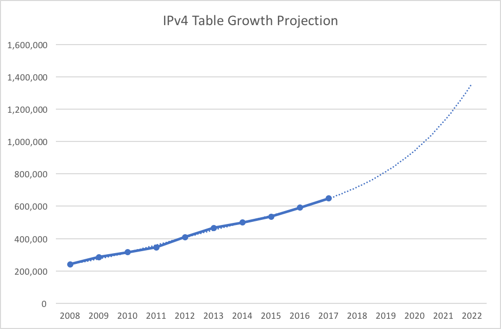
IPv4 Table Size Projection
As mentioned previously, IPv4 table size continues its rapid expansion, demonstrating approximately 10% year-over-year growth over the past few years.
2009 to 2017 IPv4 Table Size Growth:
2009
2010
2011
2012
2013
2014
2015
2016
2017
Table
Size (Thousand Routes)
286
316
345
409
466
499
536
591
648
Year
over
Year (%)
18
10
9
19
14
7
7
10
10
2017 IPv4 Table Size Growth to Date:
Month
Jan
Feb
Mar
Apr
May
Jun
Jul
Aug
Sep
Oct
Table Size (Thousand Routes)
648
653
663
663
673
676
679
684
688
691
Month over Month (%)
0.7
1.5
0.1
1.5
0.5
0.4
0.7
0.5
0.5
Compared to January (%)
0.7
2.2
0.3
3.9
4.4
4.8
5.5
6.1
6.6
Our statistical model shows that if this growth continues, global Internet table will surpass 1 Million entries sometime in 2020.
IPv4 BGP Table Size Growth Projection
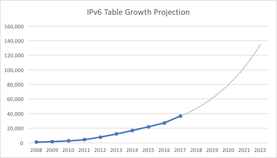
IPv6 Table Size Projection
As IPv6 gets adopted by Service Providers and Enterprises, IPv6 table size is also expected to continue to raise. The current year-over-year growth is about 30% with no signs of deceleration.
2009 to 2017 IPv6 Table Size Growth:
2009
2010
2011
2012
2013
2014
2015
2016
2017
Table Size (Thousand Routes)
1.6
2.5
4.1
7.7
12
17
22
27
37
Year
over
Year (%)
65
52
65
86
56
41
29
25
35
2017 IPv6 Table Size Growth to Date:
Jan
Feb
Mar
Apr
May
Jun
Jul
Aug
Sep
Oct
Table Size (Thousand Routes)
36
37
38
39
40
40
42
43
44
44
Month over Month (%)
2.7
3.0
0.8
2.2
1.1
3.1
2.7
2.0
0.4
Compared to January (%)
2.7
5.7
6.6
9.0
10.3
13.7
16.7
19.0
19.5
While IPv6 table is not expected to grow to the same size as IPv4 table due to much bigger initial block allocations by the registries, ongoing IPv6 adoption will nonetheless lead to the table size increase.
IPv6 BGP Table Size Growth Projection
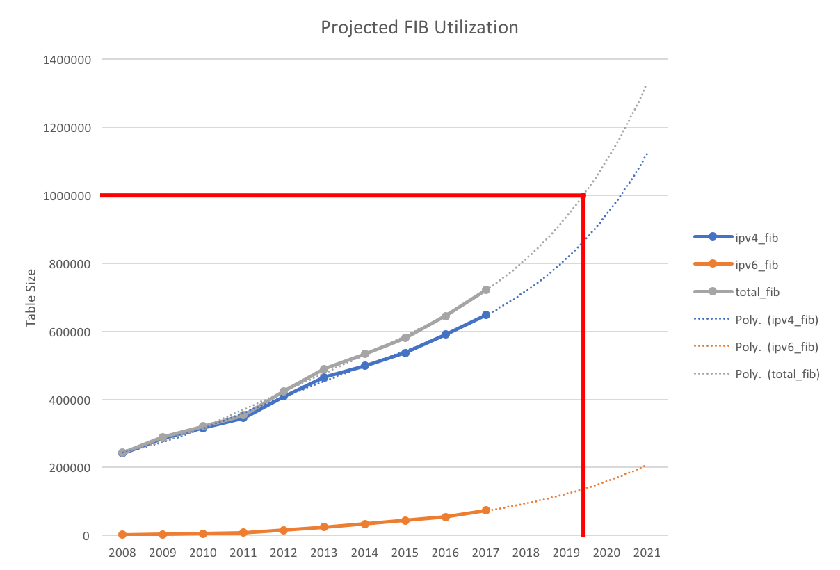
FIB Utilization
IPv4 and IPv6 table size increases will translate into FIB size increase. The actual impact on your router will depend on a specific vendor’s implementation. In the best-case scenario, you will observe one-to-one correlation between the combined size of IPv4 and IPv6 tables and FIB table. More common scenario might be IPv6 entries using twice as much space as IPv4 entries. This later scenario is depicted below:
FIB Size Growth Projection
As you can deduce from the graph, routers that are capable of supporting 1Mln routes, will run out of FIB space sometime in 2019. In fact, you might run into problems much earlier than that, if you have
Large number of disaggregated internal routes, such as loopbacks, point-to-point IPs and customer routes
BGP policy allowing to accept long (>24) prefixes from external peers
Extensive public and private peering with partners who might advertise more specific routes not otherwise visible in the public Internet
Provide other services that require FIB space, such as Mutlicast, MPLS VPN, L2 VPN, etc.
What to expect
Assuming that the FIB size of your Internet-facing router is limited by 1 Mln entries, you can expect to run into issues sometime in 2019. The actual impact will depend on the platform in use. Some systems might attempt to fall back to RE-based forwarding for the destinations which could not be programmed in hardware. This might lead to high CPU utilization on the entire system and general instability of the router.
Other systems will simply drop traffic to such destinations. This scenario can manifest itself by customers unable to reach some sites on the Internet, while accessing other sites. You should monitor system logs and FIB utilization to spot the issue.
How to prepare
As an administrator, there are a few things you should do to be ready to withstand Internet size growth:
Understand your system’s FIB capacity to make sure you have enough room to accommodate expected Internet growth
If your system allows changing FIB partitioning, make sure it is set up in the most optimal way. For example, you might want to allow for up to 800K IPv4 and 100K IPv6 routes
If possible, upgrade your systems to support at least 2Mln FIB entries. This is applicable to both Routing Engine and Line Cards
If upgrade is not viable at the moment, consider inbound route-filtering to decrease the number of routes accepted from your peers. The general consensus is that you can safely drop all IPv4 /25 and longer prefixes while maintaining full reachability of Internet destinations.
Conclusion
Internet global routing table continues to grow with no signs of slowing down. The major contributor to this growth is an ongoing IPv4 disaggregation, as well as a proliferation of IPv6 Internet. As a network administrator, you need to be prepared to protect your network from negative consequences of this growth by optimizing your routing policies and upgrading physical infrastructure.